In plain English
Imagine you need to find the closest city to an arbitrary point on a world map. You don't start by checking every city. You zoom out, pick the right continent, then the right country, then the right region, and only then do you zoom in and compare the handful of candidates nearby. That multi-scale drill-down is exactly the idea behind HNSW — Hierarchical Navigable Small World graphs.
HNSW is the indexing algorithm that most vector databases use under the hood. When you call a similarity search on Pinecone, Qdrant, Weaviate, pgvector, Milvus, or Redis, there's a good chance HNSW is doing the actual work. It organises your embeddings into a layered graph — the "hierarchy" in the name — so that search can jump straight to the right neighbourhood instead of inspecting every vector.
The word navigable small world comes from network science. In a small-world graph, any node can reach any other node in a surprisingly small number of hops — the same property that makes social networks feel connected ("six degrees of separation"). HNSW stacks multiple small-world layers on top of each other, with each higher layer acting as a coarse long-range express route that rapidly narrows the search space before the algorithm drops into the fine-grained bottom layer.
Why it matters for builders
The raw problem is that finding the closest embedding to a query vector is, without an index, an O(n) operation — you compare the query to every vector in the dataset. For 10 million 1,536-dimension OpenAI embeddings (about 60 GB of floats), a single exact-search query computes 10 million cosine distances. On a modern CPU that might take several seconds. HNSW cuts the same query to sub-linear time — often under 5 milliseconds — because it visits only a tiny fraction of the dataset.
For anyone building on embeddings, the practical implications are large:
- RAG pipelines. Every user message triggers a retrieval step that must finish before the LLM can reply. An HNSW index is what keeps that step under 20 ms even as your document corpus grows to millions of chunks.
- Semantic search and recommendations. Returning the 10 most similar products, articles, or songs from a catalogue of 50 million items in real time requires HNSW — brute-force search simply can't keep up at that scale.
- Dynamic datasets. Unlike IVF (the other common ANN algorithm), HNSW supports incremental inserts without any retraining or full rebuild. You can add new vectors continuously and search them immediately.
- Parameter intuition. Every managed vector database exposes HNSW's three knobs — M, efConstruction, efSearch — often with opaque defaults. Knowing what they actually control is the difference between a system that silently degrades at scale and one you've deliberately tuned.
HNSW is not always the right choice — for very large, mostly-static corpora where memory is tight, IVF-PQ can store 10 billion vectors on a single server that HNSW cannot. But for the vast majority of production AI applications — RAG, semantic search, recommendation, image retrieval — HNSW is the default for good reason.
How it works
HNSW builds a multi-layer graph. Every vector lives in the bottom layer (layer 0), which is a dense proximity graph connecting each node to its M nearest neighbours. Above it, a probabilistically selected subset of vectors also appear in layer 1, with longer-range connections. A smaller subset appears in layer 2, and so on until the top layer contains just a handful of nodes connected by the longest possible links.
The skip-list analogy
The layer structure mirrors a probabilistic skip list — a data structure where each element is promoted to higher express lanes with exponentially decaying probability. In HNSW, each vector is assigned a maximum layer by drawing from a geometric distribution: most vectors land only in layer 0, some reach layer 1, a few reach layer 2, and so on. This produces an exponentially thinning hierarchy that is exactly what makes top-down navigation efficient.
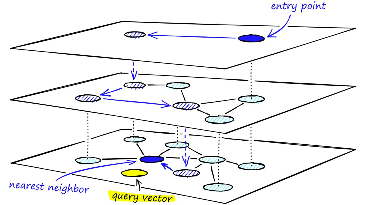
Search algorithm step by step
- Enter at the top. The algorithm starts at a fixed entry point in the highest layer.
- Greedy descent. At each layer, it greedily hops to whichever connected node is closest to the query vector, repeating until it finds a local minimum at that layer.
- Drop one layer. The local minimum becomes the entry point for the same greedy search in the next layer down.
- Beam search at the bottom. In layer 0, instead of pure greedy traversal, the algorithm maintains a priority queue of
ef(efSearch) candidates, exploring the most promising ones until the queue stops improving. This avoids getting trapped in local minima. - Return top-k. The k closest vectors from that candidate set are the results.
Index build: inserting a new vector
When a new vector arrives, HNSW randomly assigns it a maximum layer using the geometric distribution, then inserts it into every layer from 0 up to that maximum. At each layer, a greedy search finds the efConstruction closest existing nodes, and bidirectional links are created to the best M of them. Older connections that are now suboptimal may be pruned to keep each node at most M neighbours. This is the one step that is expensive — O(M * efConstruction * log n) per insert — but it only happens at write time, and it is what produces the high-quality graph that makes searches fast.
- Sparse — few nodes
- Long-range links
- Fast coarse navigation
- Entered first at query time
- Probabilistically promoted vectors only
- Dense — every vector
- Short local links
- Precise fine-grained search
- Where beam search runs
- Where top-k is harvested
The three parameters that actually matter
HNSW exposes exactly three knobs. Understanding what each one does — and which phase it affects — is enough to tune any vector database confidently.
| Parameter | What it controls | Affects | Typical range |
|---|---|---|---|
| M | Max bidirectional links per node in the graph | Index size, recall, RAM usage | 8–64 |
| efConstruction | Candidate list size during index build | Build quality (recall ceiling), build time | 100–500 |
| efSearch (ef) | Candidate list size during queries | Recall vs. latency at query time | 50–400 |
M — graph connectivity
M is the number of bidirectional edges each node maintains in the graph. A higher M means each node is connected to more neighbours, making the graph harder to get lost in — recall improves. The cost is proportional: the index uses more RAM (roughly O(M * n) edges to store) and each insert requires more comparisons. A rule of thumb: M=16 is a sane default for 384–1,536 dimensional embeddings; push toward M=32–48 for very high-dimensional vectors or when you need 0.99 recall; drop to M=8–12 for memory-constrained deployments.
efConstruction — build-time quality
During index build, each new vector's neighbourhood is found by a beam search with a candidate list of size efConstruction. A larger list means the algorithm considers more candidates before choosing the best M neighbours — producing a better-connected graph and a higher recall ceiling. Crucially, efConstruction does not affect index size or query speed; it only affects build time and the quality of the links written. You set it once when building, not at query time. Typical values: 100 for fast builds, 200–400 when you want to maximise recall.
efSearch — the real-time recall dial
efSearch (called ef in some libraries, hnsw_ef in others) is the only parameter you can change at query time without rebuilding the index. It sets the size of the beam-search candidate list at layer 0. Larger efSearch explores more of the graph before returning results: recall goes up, latency goes up proportionally. This is the primary lever for the recall-vs-speed tradeoff. Start with efSearch = 2 * top_k and increase until you hit your recall target.
# pip install faiss-cpu numpy
import faiss
import numpy as np

dim = 1536          # OpenAI text-embedding-3-small dimension
n   = 500_000        # corpus size
k   = 10            # top-k neighbours to retrieve

np.random.seed(0)
corpus = np.random.rand(n, dim).astype("float32")
queries = np.random.rand(100, dim).astype("float32")

# Build HNSW index (M=16, efConstruction=200)
index = faiss.IndexHNSWFlat(dim, 16)   # M = 16
index.hnsw.efConstruction = 200
index.add(corpus)                       # one-time build (~minutes at this scale)

# Ground-truth via brute-force flat search
flat = faiss.IndexFlatL2(dim)
flat.add(corpus)
_, gt_ids = flat.search(queries, k)

# Measure recall at different efSearch values
for ef in [10, 32, 64, 128, 256]:
    index.hnsw.efSearch = ef
    _, hnsw_ids = index.search(queries, k)
    recall = sum(
        len(set(hnsw_ids[i]) & set(gt_ids[i])) / k
        for i in range(len(queries))
    ) / len(queries)
    print(f"efSearch={ef:4d}  recall@{k}={recall:.3f}")
You'll typically see recall climb steeply from efSearch=10 to efSearch=64, then flatten near 0.97–0.99 as efSearch reaches 128–256. The latency cost of raising efSearch from 64 to 256 is roughly 3–4x — a real tradeoff, not a free lunch.
HNSW in the databases you actually use
Every major vector database exposes HNSW, but the parameter names and defaults vary. Here's the mapping so you're never hunting through docs wondering which knob is which.
| Database | M parameter | efConstruction | efSearch | Notes |
|---|---|---|---|---|
| pgvector | m | ef_construction | hnsw.ef_search (SET) | Added in pgvector 0.5.0 (2023) |
| Qdrant | m | ef_construct | ef (per-query) | Configured per collection in JSON |
| Weaviate | maxConnections | efConstruction | ef | Set at collection creation |
| Milvus | M | efConstruction | ef | Default M=8, ef_construction=64 |
| Redis | M | EF_CONSTRUCTION | EF_RUNTIME | Part of RediSearch module |
| Faiss (library) | M in constructor | hnsw.efConstruction | hnsw.efSearch | CPU and GPU variants available |
pgvector example
-- Create the index (one-time, runs in background with CREATE INDEX CONCURRENTLY)
CREATE INDEX ON documents
  USING hnsw (embedding vector_cosine_ops)
  WITH (m = 16, ef_construction = 200);

-- Tune efSearch at query time (session-level)
SET hnsw.ef_search = 100;

-- Nearest-neighbour query
SELECT id, content
FROM documents
ORDER BY embedding <=> '[0.12, 0.34, ...]'::vector
LIMIT 10;Qdrant example
from qdrant_client import QdrantClient
from qdrant_client.models import Distance, VectorParams, HnswConfigDiff

client = QdrantClient(":memory:")

client.create_collection(
    collection_name="docs",
    vectors_config=VectorParams(size=1536, distance=Distance.COSINE),
    hnsw_config=HnswConfigDiff(
        m=16,
        ef_construct=200,
        full_scan_threshold=10_000,   # use flat scan for small collections
    ),
)

# Override ef at query time
results = client.search(
    collection_name="docs",
    query_vector=query_embedding,
    limit=10,
    search_params={"hnsw_ef": 128, "exact": False},
)Going deeper
Once you're comfortable with the three core parameters, the next set of concerns involves how HNSW behaves at the edges: very large datasets, memory limits, filtered queries, and the difference between what the paper promises and what happens in production.
Memory: HNSW's main cost
HNSW stores every vector plus all its graph edges in RAM. With M=16 on a 1,536-dimension float32 corpus, expect roughly 1.5–2x the raw vector storage for the graph overhead. At 50 million vectors (about 300 GB raw), the full HNSW index can exceed 600 GB — a server-class memory requirement. This is why memory-constrained deployments use scalar quantization (SQ8) — which compresses each float32 dimension to an int8, cutting storage by 4x with minimal recall loss — or binary quantization for a 32x compression at a more significant recall cost. Milvus, Qdrant, and Weaviate all support quantized HNSW natively.
Recall degradation at scale
An HNSW index built for 1 million vectors with M=16 may drop from 0.97 recall to 0.85 when the corpus reaches 100 million. The reason: as the dataset grows, the local neighbourhood structure at layer 0 becomes a worse approximation of the true nearest-neighbour graph — nodes that were once good proxies are now crowded out by new arrivals that the original links don't reach. The fix is periodic index rebuilds with recalibrated M and efConstruction tuned to the new size. Production systems running continuous ingestion should monitor recall@k over time and schedule rebuilds when it drifts below threshold.
Filtered HNSW search
Most real queries include a metadata filter: "find the 10 most similar products in category X, priced under $50". Naive post-filtering (run ANN search, then discard non-matching results) fails under selective filters — you might retrieve 100 candidates, filter them to 2, and miss the 8 closest that the ANN window didn't reach. Modern vector databases handle this with pre-filtering (prune the graph to only eligible nodes before traversal) or by building per-segment sub-indexes. Qdrant's payload indexes and pgvector's partial index feature are implementations of this pattern. When your filter selectivity drops below about 10%, filtered ANN is one of the harder engineering problems in vector search.
HNSW vs IVF: when to choose each
- No training phase
- Incremental inserts
- Near-logarithmic search time
- High memory (graph edges)
- Best recall-per-ms in benchmarks
- Default in most vector DBs
- Requires training on representative data
- Batch-oriented; slow for live inserts
- Linear search within clusters
- Memory-efficient (especially IVF-PQ)
- Better for billions of vectors
- Preferred when RAM is the bottleneck
For most production RAG systems, semantic search services, and recommendation engines in 2025-2026, HNSW is the correct default. It requires no training data, supports live writes, and delivers consistently high recall. Switch to IVF-PQ only when your dataset reaches hundreds of millions of vectors and you cannot afford the memory overhead — or when you're specifically using FAISS on GPU for ultra-high-throughput batch workloads.
The original paper and beyond
Malkov and Yashunin's 2018 paper (arxiv:1603.09320) remains the definitive reference. Recent research (2024–2025) has explored hub nodes — the small fraction of highly-connected nodes in HNSW's bottom layer that carry a disproportionate share of search traffic and can become bottlenecks under concurrent load. Work like NSG (Navigating Spreading-out Graph) and DiskANN (from Microsoft Research) addresses scaling HNSW-style graphs to tens of billions of vectors by storing parts of the graph on NVMe SSD rather than in RAM. DiskANN is available in Azure AI Search and influenced pgvectorscale's streaming DiskANN index. These are the directions active research is pushing as vector workloads continue to scale.
FAQ
What does HNSW stand for and who invented it?
HNSW stands for Hierarchical Navigable Small World. It was invented by Yury Malkov and Dmitry Yashunin, first published as an arXiv preprint in 2016 and formally published in IEEE Transactions on Pattern Analysis and Machine Intelligence in 2018. The name reflects the algorithm's two key ideas: a multi-layer hierarchy of graphs, and navigable small-world connectivity where any node can reach any other in a small number of hops.
What is the difference between M, efConstruction, and efSearch in HNSW?
They control three different phases. M sets how many bidirectional links each node keeps in the graph — it determines the graph structure and is fixed at index creation. efConstruction is the candidate list size used during index build — larger values produce a better-connected graph but take more time to build. efSearch (also called ef) is the candidate list size used during queries — it's the only parameter you can change without rebuilding the index, and it's the main dial for tuning recall vs. latency at query time.
Why does HNSW use more memory than other vector indexes?
HNSW stores not just the raw vectors but the entire graph structure — all the bidirectional edges between nodes across every layer. With M=16, each vector keeps 16 links per layer it appears in. This graph overhead typically adds 50–100% on top of raw vector storage. In contrast, IVF-PQ compresses vectors with product quantization and only stores cluster centroids for the graph, using far less RAM at the cost of lower recall.
Can I add new vectors to an HNSW index without rebuilding it?
Yes — incremental inserts are one of HNSW's key advantages over IVF. Each new vector is inserted by running a greedy search to find its neighbourhood, creating bidirectional links, and pruning excess connections. The insert cost is O(M * efConstruction * log n) per vector. There's no batch training step or full rebuild required. This makes HNSW well-suited for applications with continuous ingestion, like live document stores or real-time recommendation systems.
What recall can I expect from HNSW at default settings?
With typical defaults (M=16, efConstruction=200, efSearch=100) on million-scale datasets, HNSW usually achieves recall@10 of 0.95–0.98. Recall depends heavily on your data's intrinsic dimensionality, the distance metric, and how evenly distributed your vectors are. High-dimensional sparse vectors (like BM25-style embeddings) tend to be harder than dense semantic embeddings. Always measure recall against your actual query distribution, not synthetic benchmarks.
How is HNSW different from a standard k-NN graph?
A standard k-nearest-neighbour graph connects each node to its k closest neighbours, but it has no hierarchy — searches traverse the same dense layer from start to finish, making it easy to get trapped in local neighbourhoods far from the query. HNSW adds a multi-layer hierarchy of progressively sparser graphs, which acts like a highway system: the top layers allow fast long-range navigation to the right region of the space before descending to the dense bottom layer for precise local search. This is what gives HNSW its near-logarithmic search time.