In plain English
A modern transformer is a tall stack of nearly identical layers — 32, 80, sometimes over a hundred of them, piled on top of each other. Each layer nudges the data a little closer to a good answer. The obvious worry: if you stack a hundred layers and each one can distort the signal, won't the message turn to mush long before it reaches the top? In early deep networks, that is exactly what happened.
Two unglamorous components keep this from breaking: the residual connection (also called a skip connection) and layer normalization (layer norm for short). They never get the spotlight that attention does, but without them you simply cannot train a deep transformer. They are the plumbing and the structural beams — invisible when they work, catastrophic when they fail.
Here is the everyday picture. Imagine a long assembly line where each station improves a product. A residual connection is a conveyor belt running alongside every station: the original item always rolls past untouched, and each station only adds its small improvement on top. If a station has nothing useful to contribute, the item still reaches the end intact — nothing is lost. Layer norm is the quality-control checkpoint between stations that resizes every item back to a standard scale, so one overenthusiastic station can't send giant or tiny parts down the line and jam everything downstream.
Why it matters
To see why these two pieces matter, you have to understand how a deep network learns. Training works by backpropagation: the model measures its error at the top, then pushes a correction signal — the gradient — backward through every layer so each one knows how to adjust. That backward signal has to survive the trip from the last layer all the way to the first.
In a plain deep stack, the gradient gets multiplied by something at every layer on the way down. Multiply by numbers slightly less than 1 a hundred times and the signal shrinks toward zero — the vanishing gradient problem, where early layers barely learn at all. Multiply by numbers slightly more than 1 and it blows up — the exploding gradient problem, where training diverges into garbage. Either way, deep networks were historically unstable and untrainable, which is the wall these tricks were invented to break through.
- Residual connections fix gradient flow. By adding each layer's input back to its output, they create a direct highway for the gradient to travel down the stack untouched. The signal reaches the bottom layers with full strength, so every layer actually learns.
- Layer norm fixes activation scale. It rescales the numbers flowing forward through the network so they stay in a sane, consistent range. This keeps the math well-behaved, makes training far less sensitive to the learning rate, and lets you use larger steps without blowing up.
- Together they unlock depth. Depth is one of the main levers behind scaling laws — bigger, deeper models are more capable. Without stable gradient flow and stable activations, you could not stack the dozens of layers that today's frontier LLMs depend on.
So if attention is the part of the transformer that does the interesting thinking, residuals and layer norm are the part that lets you stack that thinking deep enough to be powerful. They are why how LLMs are trained at this scale is even possible.
How it works
The residual connection: add the input back
A residual connection is almost embarrassingly simple. A normal layer computes output = Layer(x). A residual layer computes output = x + Layer(x). That is the whole idea: take whatever the layer produced and add the original input back on top of it.
Why does this small change matter so much? Because the layer no longer has to reproduce the entire signal from scratch — it only has to learn the change, the residual (hence the name). If the best thing a layer can do is nothing, it just learns to output near-zero, and x + 0 = x passes the input straight through. That makes adding a useless layer harmless instead of harmful, which is exactly what you want when you are stacking a hundred of them.
The deeper payoff is in the backward pass. Because addition splits the gradient and sends a copy down both branches, the residual path forms an uninterrupted highway from the top of the network to the bottom. The gradient can always flow back along that highway at full strength, no matter how deep the stack — which is precisely the cure for vanishing gradients.
Layer norm: rescale every token to a standard size
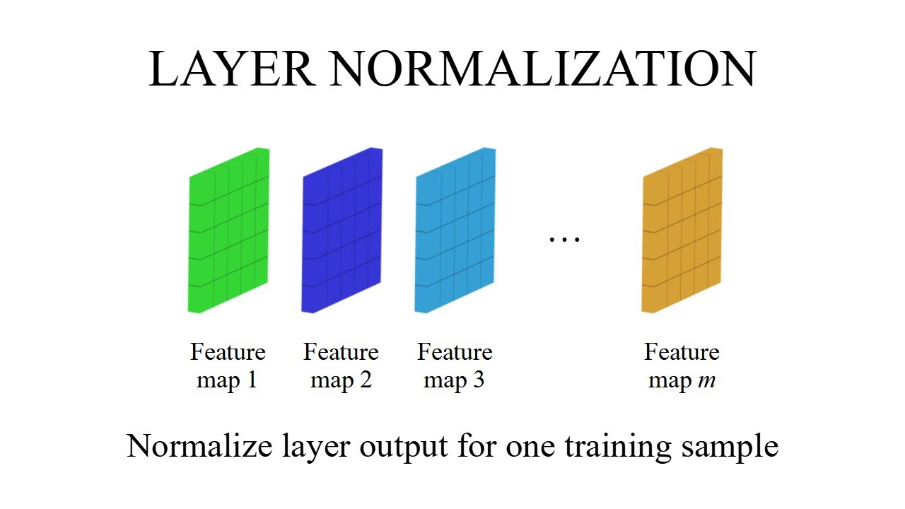
Layer normalization works on each token's vector independently. For a single token's vector of numbers, it computes the mean and the spread (standard deviation) across that vector, subtracts the mean, and divides by the spread. The result is a vector recentered to roughly zero mean and unit scale. Two tiny learnable knobs — a scale (gamma) and a shift (beta) — then let the model stretch and move that normalized vector if it needs to, so normalization never removes useful information, it just standardizes the range.
Now put the two together. Every transformer layer has two sub-blocks — attention and a small feed-forward network — and each sub-block is wrapped in its own residual connection with a layer norm attached. The data flows like this:
Stack that block over and over — attention sub-block, then feed-forward sub-block, repeated dozens of times — and you have the body of a transformer. The residual highway threads straight through all of it, and a layer norm sits at the entrance of every sub-block to keep the numbers tame.
Pre-norm vs post-norm
There is one design choice that quietly shapes whether a deep transformer trains smoothly: where you put the layer norm relative to the residual connection. There are two arrangements, and the field shifted decisively from one to the other.
| Post-norm (original) | Pre-norm (modern default) | |
|---|---|---|
| Formula | LayerNorm(x + Layer(x)) | x + Layer(LayerNorm(x)) |
| Norm sits | After the residual add | Before the sub-block, inside the residual |
| Residual highway | Interrupted by norm at every layer | Clean, unbroken path top to bottom |
| Deep-stack stability | Fragile; often needs careful warmup | Stable even at great depth |
| Used by | The original 2017 transformer | Most modern LLMs |
The original transformer used post-norm: do the sub-block, add the residual, then normalize the sum. It works, but the normalization sits on the residual highway itself, so the clean gradient path gets squeezed at every layer. Training very deep post-norm models is touchy and usually requires a careful learning-rate warmup schedule to avoid blowing up early.
Pre-norm moves the layer norm to the start of each sub-block, so it normalizes the input before the computation and the residual add happens last and untouched. This leaves the residual highway perfectly clean from top to bottom, which makes deep stacks dramatically more stable to train. That is why nearly every large transformer built in recent years uses pre-norm — it is the practical default.
- Norm after the add
- Norm sits on the residual path
- Harder to train deep
- Often needs warmup
- Original transformer
- Norm before the sub-block
- Residual path stays clean
- Stable at great depth
- Forgiving learning rates
- Modern LLM default
A worked feel for the numbers (and RMSNorm)
To make layer norm concrete, here is the entire operation on a single token's vector — no framework, just the math written out. This is what runs at the start of every sub-block, for every token, in every layer.
import numpy as np

def layer_norm(x, gamma, beta, eps=1e-5):
    # x is ONE token's feature vector, e.g. shape (d_model,)
    mu = x.mean()                 # mean across the features
    var = x.var()                 # spread across the features
    x_hat = (x - mu) / np.sqrt(var + eps)   # recenter + rescale
    return gamma * x_hat + beta    # learnable scale and shift

# A wildly-scaled activation vector...
x = np.array([12.0, -40.0, 3.0, 88.0])
gamma = np.ones(4)   # start as no-op; learned during training
beta  = np.zeros(4)

print(layer_norm(x, gamma, beta))
# -> values recentered to ~zero mean, ~unit spread,
#    no matter how large or small the inputs were
The point: whatever crazy magnitudes the previous layer produced, layer norm hands the next sub-block a vector in a predictable range. The gamma and beta knobs (and the order of operations) are the only things the model tunes; the recentering itself is fixed arithmetic.
Many recent LLMs use a lighter cousin called RMSNorm (root-mean-square normalization). It skips the mean-subtraction step and only rescales by the vector's root-mean-square magnitude. It drops the beta shift and the mean computation, which makes it cheaper to run, and in practice it works about as well — so it has become a popular swap in large models where every saved operation counts at scale.
Common pitfalls and misconceptions
These components are simple, which makes them easy to misunderstand. A few traps worth avoiding:
- Confusing layer norm with batch norm. Batch normalization rescales using statistics gathered across the batch of examples. Layer norm rescales using statistics within one token's own features. Transformers use layer norm precisely because it does not depend on batch size or sequence length, which keeps training and inference behavior identical.
- Thinking the residual is optional polish. It is not a minor optimization. Remove residual connections from a deep transformer and the gradient vanishes — the model essentially refuses to train past a handful of layers. The skip path is load-bearing.
- Assuming layer norm changes the meaning of the data. It standardizes scale, not content. The learnable scale and shift let the model recover any range it actually needs, so normalization adds stability without throwing away information.
- Ignoring the pre-norm vs post-norm choice on deep models. On a shallow network it barely matters. On a deep stack it is the difference between a run that converges smoothly and one that diverges or demands fragile warmup tuning.
Going deeper
Once the basics click, here are the nuances and directions that matter in real systems.
The final norm and warmup interplay. Pre-norm transformers add one extra layer norm at the very top of the stack, after the last block, before the output projection — because with pre-norm the residual stream is never normalized on its own, so it needs a final cleanup. And while pre-norm is forgiving, training still often uses a brief learning-rate warmup, because the earliest steps are when scale instabilities are most likely to bite.
The residual stream as a shared workspace. A useful mental model from interpretability research: the residual highway running through the whole network is a kind of shared bus. Every sub-block reads from it and writes a small update back onto it, rather than replacing it. This view explains why you can sometimes add, remove, or reorder layers with surprisingly graceful degradation — each one is contributing an increment, not the whole signal.
Interaction with efficiency tricks. These components sit alongside the rest of the modern transformer toolkit. Efficient attention implementations like FlashAttention change how the attention sub-block is computed without touching the residual-and-norm wrapper around it. And in a mixture-of-experts model, the feed-forward sub-block is swapped for a routed set of experts — but it is still wrapped in the same residual connection and normalization. The plumbing stays constant even as the computation inside it changes.
Precision matters for norms. Large models train in low-precision number formats to save memory and speed up the GPUs that run them. Normalization statistics — the mean and variance — are usually computed in higher precision even when the rest of the layer runs low, because tiny errors there can destabilize the whole stack. It is a small detail that quietly protects training stability at scale.
The durable takeaway: residual connections and layer normalization are not exciting, but they are the reason the elegant idea of stacking attention layers actually works at the depths modern models require. Master attention to understand what a transformer thinks; master residuals and norms to understand why it can think deeply at all. From here, the natural next steps are how attention works and the broader picture of how LLMs work.
FAQ
What are residual connections in a transformer?
A residual (or skip) connection adds a layer's input back to its output, computing x + Layer(x) instead of just Layer(x). This lets the original signal pass through untouched and gives the training gradient a clean highway to flow back through deep stacks, which is what makes networks with dozens or hundreds of layers trainable.
Why do transformers use layer normalization?
Layer norm rescales each token's feature vector to a standard range (roughly zero mean, unit spread) before or after each sub-block. This keeps activation magnitudes stable as data flows through many layers, makes training far less sensitive to the learning rate, and prevents the numbers from exploding or collapsing in a deep stack.
What is the difference between pre-norm and post-norm?
Post-norm (the original transformer) normalizes after the residual add: LayerNorm(x + Layer(x)). Pre-norm (the modern default) normalizes before the sub-block: x + Layer(LayerNorm(x)), leaving the residual path clean. Pre-norm is much more stable to train at great depth, which is why nearly all recent large models use it.
What is the difference between layer norm and batch norm?
Layer norm normalizes across the features of a single token, independently of other examples. Batch norm normalizes across the whole batch of examples per feature. Transformers prefer layer norm because it does not depend on batch size or sequence length, so it behaves identically during training and inference.
What is RMSNorm and how is it different from LayerNorm?
RMSNorm is a lighter variant that rescales a vector by its root-mean-square magnitude only, skipping the mean-subtraction and the shift term that LayerNorm uses. It is cheaper to compute and works about as well, so many recent large language models use it in place of standard layer norm.
Can you train a deep transformer without residual connections?
In practice, no. Without the residual highway, the gradient vanishes as it travels back through many layers, so the early layers barely learn and the model fails to train beyond a handful of layers. Residual connections are load-bearing, not an optional optimization.