In plain English
An embedding is a long list of decimal numbers that captures the meaning of a piece of text, an image, or a product. A typical one has 768 or 1536 numbers, each stored as a 4-byte float. A single 1536-dimension vector is therefore about 6 KB. That sounds tiny — until you have a billion of them. A billion vectors at 6 KB each is roughly 6 terabytes of RAM, which no single machine can hold and few budgets can afford.
Product quantization (PQ) is a compression trick that shrinks each of those vectors by 10x to 30x or more, so the whole collection fits in memory and search stays fast. It does this by approximating every vector with a short code — often just 16 to 64 bytes — instead of the full list of floats.
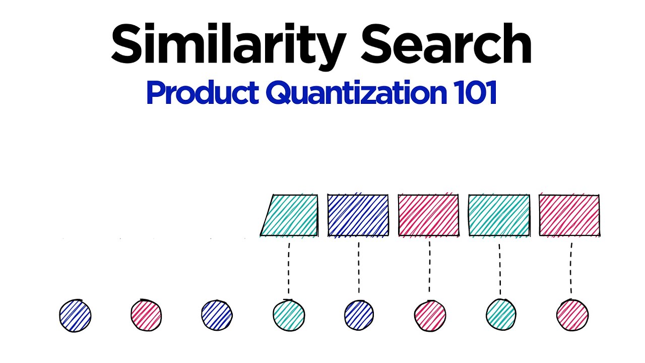
Here is the everyday analogy. Imagine you describe thousands of outfits and you must store each description in as few characters as possible. Instead of writing out every garment in full, you build three small catalogues: 32 standard tops, 32 standard bottoms, and 32 standard pairs of shoes. Now any outfit becomes three small numbers — "top #14, bottom #07, shoes #22" — three bytes instead of three paragraphs. You lose the exact shade and fit, but you keep enough to tell outfits apart. Product quantization does the same to a vector: it splits the vector into chunks, builds a tiny catalogue (a codebook) of typical chunks, and replaces each chunk with the ID of its closest catalogue entry.
Why it matters
Vector search has one brutal constraint: to be fast, the vectors need to live in RAM, not on disk. The moment you spill to disk, latency jumps from microseconds to milliseconds, and at scale that is the difference between a usable product and a stalled one. Memory, not CPU, is usually the wall you hit first.
Product quantization moves that wall. Compressing vectors 20x means a dataset that needed 600 GB of RAM now needs 30 GB — the difference between a rack of servers and a single box. For anyone running semantic search over tens of millions of documents, or a recommendation system over a billion items, PQ is often what makes the project financially possible at all.
- Memory cost. This is the headline win. Storing 1-byte codes instead of 4-byte floats, and using far fewer of them, cuts RAM by an order of magnitude or more — and RAM is the dominant cost of an in-memory index.
- Faster distance math. Comparing a query to a compressed code uses small precomputed lookup tables instead of a full dot product over hundreds of dimensions. Each comparison becomes a handful of table reads and adds, so you scan more candidates per millisecond.
- Scale that was impossible. Billion-vector indexes on a single machine simply do not exist without compression. PQ (and its relatives) are how libraries like FAISS and systems like ScaNN reach that scale.
The catch — and there is always a catch — is recall. PQ stores an approximation, so the distances it computes are estimates. Sometimes the true nearest neighbor gets ranked slightly lower and falls out of your top results. The entire craft of using PQ well is buying huge memory savings while giving up as little accuracy as you can tolerate.
How it works
Product quantization has two phases, just like building any search index. Training learns the codebooks once, up front, from a sample of your vectors. Encoding then converts every vector into a compact code. At query time, you estimate distances directly from those codes.
Step 1 — split each vector into sub-vectors
Take a 1536-dimension vector and chop it into, say, 96 contiguous chunks of 16 dimensions each. Every chunk is a small sub-vector. The number of chunks is usually written as m, so here m = 96. Each original vector is now a sequence of 96 little sub-vectors instead of one big vector.
Step 2 — learn a codebook for each chunk position
For each of the m chunk positions, gather that chunk from many training vectors and run k-means clustering on it to find a fixed number of representative points — typically 256 of them, because 256 values fit in exactly one byte. Those 256 representative sub-vectors are the codebook for that position. You end up with m separate codebooks, one per chunk, each holding 256 centroids.
Step 3 — encode every vector as a list of codebook IDs
To compress a vector, walk through its m chunks. For each chunk, find the nearest centroid in that chunk's codebook and record its ID (a number from 0 to 255 — one byte). The whole vector becomes m bytes: with m = 96, that is 96 bytes, down from 1536 floats × 4 bytes = 6144 bytes. A 64x reduction in this example, before any index overhead.
Step 4 — estimate distance from the codes
Here is the clever part. When a query arrives, you split the query into the same m chunks. For each chunk position, you precompute the distance from the query's sub-vector to all 256 centroids in that codebook, and store those in a small lookup table. That is m × 256 distances computed once per query.
Now, to estimate the distance between the query and any stored vector, you do not touch the original floats at all. You read each of the stored vector's m byte codes, look up the matching precomputed distance, and add them together. A full distance becomes m table lookups and m additions — no multiplications, no float vectors. This is called asymmetric distance computation (the query stays full-precision while the database is quantized), and it is why PQ scans are so fast.
import numpy as np

# codebooks[j] holds 256 centroids for chunk j  -> shape (m, 256, dsub)
# query is split into m sub-vectors            -> shape (m, dsub)

def build_lookup(query_subs, codebooks):
    # One (m, 256) table of squared distances, computed once per query.
    m, K, _ = codebooks.shape
    table = np.empty((m, K), dtype=np.float32)
    for j in range(m):
        diff = codebooks[j] - query_subs[j]      # (256, dsub)
        table[j] = np.sum(diff * diff, axis=1)   # (256,)
    return table

def estimate_distance(code, table):
    # code is m bytes of centroid IDs for one stored vector.
    # Sum one looked-up distance per chunk -- no float math over the vector.
return sum(table[j, code[j]] for j in range(len(code)))IVFPQ: riding on top of IVF
PQ on its own makes each vector cheap to store and compare, but a naive search still scans every code. At a billion vectors, even cheap comparisons add up. The standard production fix is to combine PQ with an inverted file index (IVF) — the pairing is so common it has its own name: IVFPQ.
IVF is a coarse first pass. Before any PQ, you cluster all the vectors into many buckets (say 4096 of them) and remember which bucket each vector landed in. At query time you find the few buckets nearest the query and only search inside those, ignoring the rest. This is a form of approximate nearest neighbor search: you trade a small chance of missing the true answer for scanning a tiny fraction of the data.
So IVF cuts how many vectors you look at, and PQ cuts how much each one costs to store and compare. Together they make billion-scale search fit on one machine. A common final touch is a rerank step: take the few hundred best candidates the PQ estimate found, fetch their full vectors (kept on disk or recomputed), and re-score those with exact distance. The expensive exact math runs on a tiny shortlist, recovering most of the accuracy PQ gave up while still scanning the whole index cheaply.
The memory math and the knobs
PQ has two main dials, and understanding them is most of using it well. They are m, the number of chunks (= bytes per code), and nbits, the bits per chunk code (almost always 8, giving 256 centroids per codebook). The compressed size of one vector is simply m × nbits / 8 bytes.
| Setting | Bytes per vector | Vs. 1536 float32 (6144 B) | Effect on recall |
|---|---|---|---|
| m = 192, 8 bits | 192 B | 32x smaller | Highest recall, least compression |
| m = 96, 8 bits | 96 B | 64x smaller | Strong balance, common default |
| m = 48, 8 bits | 48 B | 128x smaller | Aggressive; recall starts dropping |
| m = 24, 8 bits | 24 B | 256x smaller | Tiny; only for huge, recall-tolerant sets |
The trend is clear: more chunks means finer approximation and higher recall, but bigger codes and less compression. Fewer chunks means tinier codes but a coarser, lossier approximation. There is no universally right setting — it depends on how much memory you have, how much recall your product needs, and the dimensionality of your embeddings. The usual practice is to fix a memory budget, then turn up m as high as that budget allows.
Two practical requirements fall out of the math. First, the embedding dimension should divide evenly by m, so the chunks are equal in size. Second, you need enough training vectors to learn 256 meaningful centroids per chunk — a few tens of thousands of samples is a reasonable floor. Train on too little data and the codebooks will not represent your real vectors, quietly hurting recall no matter how you set m.
PQ vs scalar and binary quantization
Product quantization is one of several ways to compress vectors, and it helps to see where it sits. The other two you will meet most are scalar quantization and binary quantization. They differ in how aggressively they compress and how much accuracy they keep.
- Splits vector into chunks
- Learns a codebook per chunk
- 10-30x+ smaller
- Needs training on your data
- Best ratio of size to recall
- Compresses each number alone
- float32 to int8 per dimension
- About 4x smaller
- No codebook, trivial to apply
- Mild, safe accuracy loss
- Each dimension becomes 1 bit
- Sign of the value only
- Up to 32x smaller
- Distance via fast XOR
- Largest accuracy hit; rerank needed
Scalar quantization is the easy first step: round each float to an 8-bit integer, get a clean 4x reduction with little fuss and small accuracy loss, and require no training. Binary quantization is the extreme: keep only whether each number is positive or negative, one bit per dimension, which is brutally compact and lets you compare vectors with bitwise XOR — but you almost always have to rerank the survivors with full precision to recover usable accuracy.
Product quantization sits between them in effort and ahead of both in efficiency: for a given memory budget it generally preserves more accuracy than binary and compresses far harder than scalar, at the cost of a training step and more moving parts. A common modern pattern is to combine ideas — for example, binary or PQ codes for a fast first pass, then a precise rerank — rather than treating them as mutually exclusive.
Going deeper
Once the basics click, several details separate a PQ index that works in a demo from one that holds up in production.
Recall is measured, not assumed. Never ship a PQ index on faith. Build a small ground-truth set by running exact (brute-force) search on a sample of queries, then check what fraction of those true neighbors your PQ index returns — this is recall@k. Tune m, the number of IVF buckets you probe (nprobe), and your rerank depth against that number. The right configuration is the one that hits your recall target at your memory budget, and it can only be found empirically.
Asymmetric beats symmetric. Always keep the query vector at full precision and compare it against the quantized database codes (asymmetric distance), rather than quantizing the query too. Quantizing both sides is slightly cheaper but throws away accuracy for no real gain, since the query side is computed only once anyway.
PQ approximates distance, not identity. Because two different vectors can round to the same set of centroid IDs, PQ can never tell you a vector is exactly a certain item — only that it is close. For tasks that need exact matches (deduplication, lookups by ID) PQ is the wrong tool. It is built for nearest-neighbor search, where "close enough" is the whole point.
It rides on top of your index, not instead of it. PQ is a storage-and-distance technique; you still need an indexing structure — IVF buckets, an HNSW graph, or a flat scan — to decide which vectors to compare. Most vector databases expose PQ as a configuration option on top of their index rather than as a standalone mode, so the practical question is usually "IVF + PQ with what m and nprobe," not "PQ yes or no."
Where to go next: study how IVF and graph indexes choose candidates in approximate nearest neighbor search, make sure you understand the distance metric your embeddings expect via cosine similarity vs dot product, and read the FAISS documentation, where IVFPQ and OPQ are first-class building blocks you can configure with a short index string.
FAQ
What is product quantization in simple terms?
It is a compression method for embedding vectors. You split each vector into several chunks, build a small catalogue (codebook) of typical chunks, and replace each chunk with the ID of its closest catalogue entry. A long list of floats becomes a handful of bytes, shrinking memory by 10-30x or more while keeping enough information to find approximate nearest neighbors.
How much memory does product quantization save?
Typically 10-30x, and more in aggressive settings. A 1536-dimension float32 vector is about 6 KB; with 96 one-byte codes it drops to 96 bytes, roughly a 64x reduction before index overhead. The exact saving is m × nbits / 8 bytes per vector, where m is the number of chunks and nbits is usually 8.
What is the difference between PQ and IVFPQ?
PQ is the compression step: it shrinks each vector and lets you estimate distances from the codes. IVF is a separate step that clusters vectors into buckets so you only search the few buckets nearest a query. IVFPQ combines them — IVF reduces how many vectors you scan, PQ reduces how costly each one is — which is the standard recipe for billion-scale search.
Does product quantization hurt search accuracy?
Yes, somewhat. Because PQ stores an approximation, the distances it computes are estimates and the true nearest neighbor can occasionally be ranked too low. You manage this by tuning the number of chunks, using OPQ, and reranking a shortlist of candidates with exact distances. The goal is to keep recall high enough for your use case at the memory budget you can afford.
How is product quantization different from binary quantization?
Binary quantization keeps only one bit per dimension (the sign of each value), so it is extremely compact and fast via XOR but loses a lot of accuracy and usually needs a rerank pass. Product quantization splits the vector into chunks and learns a codebook per chunk, which costs a training step but generally preserves more accuracy for a given size. PQ trades simplicity for a better size-to-recall ratio.
What does the 'm' parameter control in PQ?
m is the number of chunks each vector is split into, which equals the number of bytes in the compressed code when you use 8-bit codes. A larger m gives a finer approximation and higher recall but bigger codes and less compression; a smaller m gives tinier codes but a coarser, lossier approximation. The embedding dimension should divide evenly by m.